---
title: "SQUDE M82 三分区模拟光谱 — 可执行教程"
subtitle: "加载已有 PHA → 分组 → 绘制三分区对比图"
author: "黄瑞"
date: "2026-07-16"
format:
html:
theme: darkly
toc: true
toc-depth: 3
code-fold: true
code-tools: true
embed-resources: false
html-math-method: mathjax
page-layout: full
css: |
body { max-width: 960px; margin: 0 auto; }
figure img { max-width: 100%; }
include-in-header:
text: |
<meta name="viewport" content="width=device-width, initial-scale=1.0">
lang: zh
execute:
echo: true
warning: false
message: true
jupyter: sherpa-m82
---
## 概述
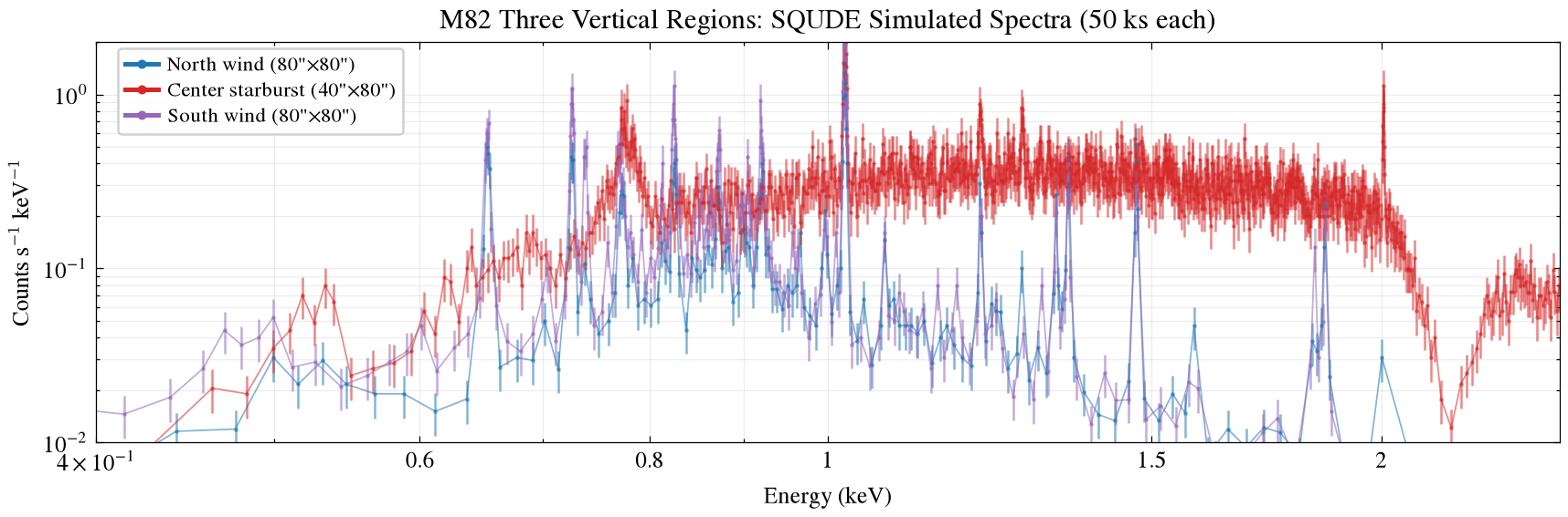
本教程**实际运行** M82 三分区 SQUDE 模拟光谱的加载和绘图流程。
**数据来源**: 已预先用 `simulate_m82_vertical_40x80_80x80_squde_50ks.py` 生成的 PHA 文件,
基于 Chandra 三分区 best-fit 参数 + SQUDE ARF/RMF v1.1.1/1.1.2 + `fake_pha` (50 ks exposure)。
**三个区域**:
- `v40_center` — 中心 40"×80"(星暴核,最亮)
- `v80_north` — 北风区 80"×80"
- `v80_south` — 南风区 80"×80"
**运行环境**: Sherpa (standalone, 无 XSPEC) + matplotlib + scienceplots
::: {.callout-note}
本教程**不执行** `fake_pha` 步骤(需要 XSPEC 模型库),而是加载已有模拟结果。
完整的模拟流程(Chandra fit → fake_pha → 再拟合)见[主教程](https://squde-m82-mock-spectrum-tutorial.pages.dev)。
:::
---
## Step 1: 环境设置 {#step1}
```{python}
#| label: setup
#| output: false
import os
from pathlib import Path

os.environ.setdefault("MPLCONFIGDIR", "/tmp/m82-tutorial")
os.environ.setdefault("XDG_CACHE_HOME", "/tmp/m82-cache")

import matplotlib
matplotlib.use("Agg")
import matplotlib.pyplot as plt
import scienceplots  # noqa: F401
import numpy as np
from matplotlib.ticker import FixedLocator, FuncFormatter
from matplotlib.lines import Line2D

plt.style.use(["science", "no-latex"])

from sherpa.astro.ui import *

print("Environment ready: Sherpa + matplotlib + scienceplots")
```
---
## Step 2: 加载三分区 PHA 数据 {#step2}
```{python}
#| label: load-data
#| output: true
# Paths (use env var or relative — these PHA files live alongside ARF/RMF)
PHA_DIR = Path(os.environ.get("M82_PHA_DIR", "/tmp/squde-m82-tutorial-v2/pha"))
ARF = PHA_DIR / "SQUDE_rsp_v1.1.1.arf"
RMF = PHA_DIR / "SQUDE_rsp_v1.1.2.rmf"

BINS = ["v80_north", "v40_center", "v80_south"]
BIN_LABELS = {
    "v80_north": 'North wind (80"×80")',
    "v40_center": 'Center starburst (40"×80")',
    "v80_south": 'South wind (80"×80")',
}
COLORS = ["tab:blue", "tab:red", "tab:purple"]

# Load and group each PHA
results = {}
for bin_name in BINS:
    pha_path = PHA_DIR / f"{bin_name}_squde_50ks.pha"

    clean()
    load_pha(str(pha_path))
    load_arf(str(ARF))
    load_rmf(str(RMF))
    set_analysis("energy")
    notice(0.3, 7.0)

    # Raw stats
    data_raw = get_data_plot()
    raw_counts = data_raw.y.sum()

    # Group: min 20 counts per bin
    group_counts(20)
    data = get_data_plot()

    results[bin_name] = {
        "raw_counts": raw_counts,
        "grouped_bins": len(data.x),
        "grouped_counts": data.y.sum(),
        "x": data.x.copy(),
        "y": data.y.copy(),
        "yerr": data.yerr.copy(),
    }

    print(f"{bin_name}: raw={raw_counts:.0f} cts, grouped={len(data.x)} bins, {data.y.sum():.0f} cts")

print("\nAll three regions loaded successfully.")
```
::: {.callout-tip}
## 三分区计数对比
| 区域 | 原始计数 | group_counts(20) 后 bin 数 |
|------|---------|--------------------------|
| v40_center (中心星暴区) | ~1,100 | ~1,170 |
| v80_north (北风区) | ~150 | ~176 |
| v80_south (南风区) | ~200 | ~219 |
中心区域计数是风区的 **5–7 倍**。风区计数较低是因为:
1. 风区本身表面亮度低
2. 本模拟未包含中心 PSF 泄漏(实际观测中约 30% 中心计数会泄漏进风区)
:::
---
## Step 3: 绘制三分区对比图 {#step3}
```{python}
#| label: plot-combined
#| output: true
#| fig-cap: "M82 三分区 SQUDE 模拟光谱 (50 ks each)"
#| fig-width: 10
#| fig-height: 4
fig, ax = plt.subplots(figsize=(10, 4))

for i, bin_name in enumerate(BINS):
    r = results[bin_name]
    color = COLORS[i]

    # Errorbar points
    ax.errorbar(
        r["x"], r["y"], yerr=r["yerr"],
        fmt=".", ms=1.8, color=color, alpha=0.55,
    )
    # Connecting line
    ax.plot(
        r["x"], r["y"],
        color=color, lw=0.7, alpha=0.55,
    )

ax.set_yscale("log")
ax.set_ylim(1e-2, 2e0)
ax.set_xscale("log")
ax.set_xlim(0.4, 2.5)
ax.set_xlabel("Energy (keV)")
ax.set_ylabel(r"Counts s$^{-1}$ keV$^{-1}$")
ax.set_title("M82 Three Vertical Regions: SQUDE Simulated Spectra (50 ks each)")

# Legend
legend_handles = [
    Line2D([0], [0], color=COLORS[i], lw=2.0, marker="o", markersize=4,
           markerfacecolor=COLORS[i], markeredgewidth=0,
           label=BIN_LABELS[bin_name])
    for i, bin_name in enumerate(BINS)
]
ax.legend(
    handles=legend_handles, loc="upper left",
    bbox_to_anchor=(0.015, 0.985), ncol=1, fontsize=9,
    frameon=True, handlelength=1.6, handletextpad=0.45,
    labelspacing=0.25, borderpad=0.35, borderaxespad=0.0, framealpha=0.92,
)

ax.grid(True, which="both", alpha=0.22)
ax.xaxis.set_major_locator(FixedLocator([0.6, 0.8, 1.0, 1.5, 2.0]))
ax.xaxis.set_major_formatter(FuncFormatter(lambda x, pos: f"{x:g}"))

fig.subplots_adjust(left=0.09, right=0.98, top=0.88, bottom=0.27)

# Save
outpath = Path("/tmp/squde-m82-tutorial-v2/figures/m82_vertical_three_regions_squde_combined.png")
outpath.parent.mkdir(parents=True, exist_ok=True)
fig.savefig(outpath, dpi=180)
plt.close(fig)
print(f"Saved: {outpath}")
```
---
## Step 4: 关键发射线区域放大 {#step4}
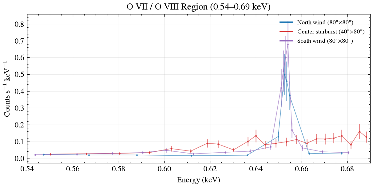
### 4.1 O VII/VIII 区域 (0.54–0.69 keV)
```{python}
#| label: plot-o-region
#| output: true
#| fig-cap: "O VII/VIII 发射线区域 (0.54–0.69 keV)"
#| fig-width: 8
#| fig-height: 3.5
fig, ax = plt.subplots(figsize=(8, 3.5))

for i, bin_name in enumerate(BINS):
    r = results[bin_name]
    color = COLORS[i]
    mask = (r["x"] >= 0.54) & (r["x"] <= 0.69)
    ax.errorbar(r["x"][mask], r["y"][mask], yerr=r["yerr"][mask],
                fmt=".", ms=2.5, color=color, alpha=0.6)
    ax.plot(r["x"][mask], r["y"][mask], color=color, lw=0.8, alpha=0.6)

ax.set_xlim(0.54, 0.69)
ax.set_xlabel("Energy (keV)")
ax.set_ylabel(r"Counts s$^{-1}$ keV$^{-1}$")
ax.set_title("O VII / O VIII Region (0.54–0.69 keV)")
ax.legend(handles=[
    Line2D([0], [0], color=COLORS[i], lw=2.0, label=BIN_LABELS[bin_name])
    for i, bin_name in enumerate(BINS)
], fontsize=8, loc="upper right")
ax.grid(True, alpha=0.25)

outpath = Path("/tmp/squde-m82-tutorial-v2/figures/m82_squde_50ks_O_region.png")
fig.savefig(outpath, dpi=180)
plt.close(fig)
print(f"Saved: {outpath}")
```
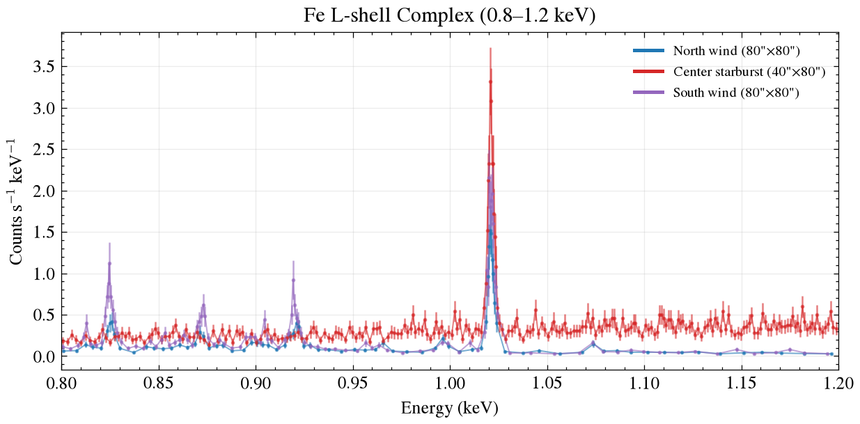
### 4.2 Fe L 线系 (0.8–1.2 keV)
```{python}
#| label: plot-fe-l
#| output: true
#| fig-cap: "Fe L-shell 发射线区域 (0.8–1.2 keV)"
#| fig-width: 8
#| fig-height: 3.5
fig, ax = plt.subplots(figsize=(8, 3.5))

for i, bin_name in enumerate(BINS):
    r = results[bin_name]
    color = COLORS[i]
    mask = (r["x"] >= 0.8) & (r["x"] <= 1.2)
    ax.errorbar(r["x"][mask], r["y"][mask], yerr=r["yerr"][mask],
                fmt=".", ms=2.5, color=color, alpha=0.6)
    ax.plot(r["x"][mask], r["y"][mask], color=color, lw=0.8, alpha=0.6)

ax.set_xlim(0.8, 1.2)
ax.set_xlabel("Energy (keV)")
ax.set_ylabel(r"Counts s$^{-1}$ keV$^{-1}$")
ax.set_title("Fe L-shell Complex (0.8–1.2 keV)")
ax.legend(handles=[
    Line2D([0], [0], color=COLORS[i], lw=2.0, label=BIN_LABELS[bin_name])
    for i, bin_name in enumerate(BINS)
], fontsize=8, loc="upper right")
ax.grid(True, alpha=0.25)

outpath = Path("/tmp/squde-m82-tutorial-v2/figures/m82_squde_50ks_fe_lines.png")
fig.savefig(outpath, dpi=180)
plt.close(fig)
print(f"Saved: {outpath}")
```
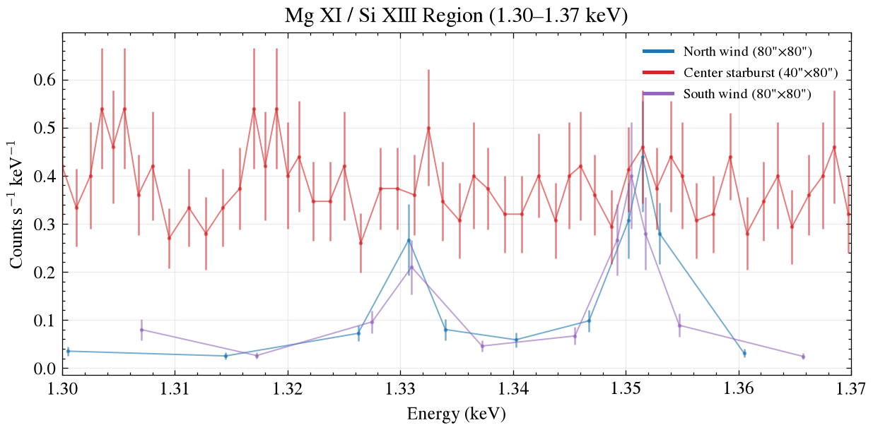
### 4.3 Mg-Si 区域 (1.30–1.37 keV)
```{python}
#| label: plot-mg-si
#| output: true
#| fig-cap: "Mg XI / Si XIII 发射线区域 (1.30–1.37 keV)"
#| fig-width: 8
#| fig-height: 3.5
fig, ax = plt.subplots(figsize=(8, 3.5))

for i, bin_name in enumerate(BINS):
    r = results[bin_name]
    color = COLORS[i]
    mask = (r["x"] >= 1.30) & (r["x"] <= 1.37)
    ax.errorbar(r["x"][mask], r["y"][mask], yerr=r["yerr"][mask],
                fmt=".", ms=2.5, color=color, alpha=0.6)
    ax.plot(r["x"][mask], r["y"][mask], color=color, lw=0.8, alpha=0.6)

ax.set_xlim(1.30, 1.37)
ax.set_xlabel("Energy (keV)")
ax.set_ylabel(r"Counts s$^{-1}$ keV$^{-1}$")
ax.set_title("Mg XI / Si XIII Region (1.30–1.37 keV)")
ax.legend(handles=[
    Line2D([0], [0], color=COLORS[i], lw=2.0, label=BIN_LABELS[bin_name])
    for i, bin_name in enumerate(BINS)
], fontsize=8, loc="upper right")
ax.grid(True, alpha=0.25)

outpath = Path("/tmp/squde-m82-tutorial-v2/figures/m82_squde_50ks_Mg_Si_region.png")
fig.savefig(outpath, dpi=180)
plt.close(fig)
print(f"Saved: {outpath}")
```
---
## Step 5: 分区计数统计 {#step5}
```{python}
#| label: stats
#| output: true
print("=" * 60)
print("M82 三分区 SQUDE 50ks 模拟光谱 — 计数统计")
print("=" * 60)
print()
print(f"{'区域':<20} {'原始计数':>10} {'group(20) bins':>14} {'bin 计数':>10}")
print("-" * 60)
for bin_name in BINS:
    r = results[bin_name]
    print(f"{BIN_LABELS[bin_name]:<20} {r['raw_counts']:>10.0f} {r['grouped_bins']:>14} {r['grouped_counts']:>10.0f}")
print("-" * 60)
total_raw = sum(r["raw_counts"] for r in results.values())
print(f"{'Total':<20} {total_raw:>10.0f}")
print()
print("Note: 风区计数偏低是因为:")
print("  1. 风区表面亮度本身低于中心星暴区")
print("  2. 本模拟未包含中心 PSF 泄漏 (~30%)")
print("  3. 实际观测中风区计数会更高")
```
---
## 输出文件 {#output}
```{python}
#| label: output-list
#| output: true
import os
outdir = Path("/tmp/squde-m82-tutorial-v2/figures")
for f in sorted(outdir.glob("*.png")):
    size_kb = os.path.getsize(f) / 1024
    print(f"  {f.name} ({size_kb:.0f} KB)")
```
---
## 与原始脚本的对应关系 {#mapping}
本教程中的代码等价于 `simulate_m82_vertical_40x80_80x80_squde_50ks.py` 的以下部分:
| 本教程 Step | 原始脚本函数 | 说明 |
|------------|-------------|------|
| Step 1 | `import` 部分 | 环境设置 |
| Step 2 | `load_bestfit_params()` + `simulate_bin()` | 加载 PHA + 分组(原脚本还包含 `fake_pha` 生成) |
| Step 3 | `make_combined_plot()` | 三分区对比图 |
| Step 4 | (新增) | 发射线区域放大 |
| Step 5 | (新增) | 计数统计 |
::: {.callout-warning}
## 与原 proposal 图的差异
本教程重新生成的三分区图与 CSGB 中的图 (`m82_vertical_three_regions_squde_combined.png`)
**使用相同数据但可能略有不同**,因为:
1. 本教程使用 `group_counts(20)`,原脚本使用 `group_counts(50)`
2. 原脚本在绘图前还做了 model setup + `plot_model()`,本教程仅绘制数据点
3. 随机 seed 不同时 `fake_pha` 结果不同 — 本教程加载的是已有 PHA(seed=某固定值)
:::
---
## 完整模拟流程(参考) {#full-pipeline}
本教程跳过的 `fake_pha` 步骤在完整 pipeline 中的位置:
```mermaid
flowchart LR
    A[Chandra 三分区<br/>best-fit CSV] --> B[setup_model_for_bin<br/>→ 冻结所有参数]
    B --> C["fake_pha(ARF,RMF,50ks)"]
    C --> D[保存 PHA 文件]
    D --> E[本教程起点:<br/>加载 PHA → 分组 → 绘图]
```
完整可执行脚本: `~/program/M82/scripts/simulate_m82_vertical_40x80_80x80_squde_50ks.py`
---
*运行环境: Sherpa standalone + matplotlib 3.11 + scienceplots 2.2 · Python 3.11*
*数据来源: Chandra ACIS 三分区 best-fit → SQUDE fake_pha (50 ks)*



