---
title: "SQUDE M82 three-region simulated spectra — executable tutorial"
subtitle: "Load existing PHA → group → plot the three-region comparison"
author: "Rui Huang"
date: "2026-07-16"
format:
html:
theme: darkly
toc: true
toc-depth: 3
code-fold: true
code-tools: true
embed-resources: false
html-math-method: mathjax
page-layout: full
css: |
body { max-width: 960px; margin: 0 auto; }
figure img { max-width: 100%; }
include-in-header:
text: |
<meta name="viewport" content="width=device-width, initial-scale=1.0">
lang: zh
execute:
echo: true
warning: false
message: true
jupyter: sherpa-m82
---
## Overview
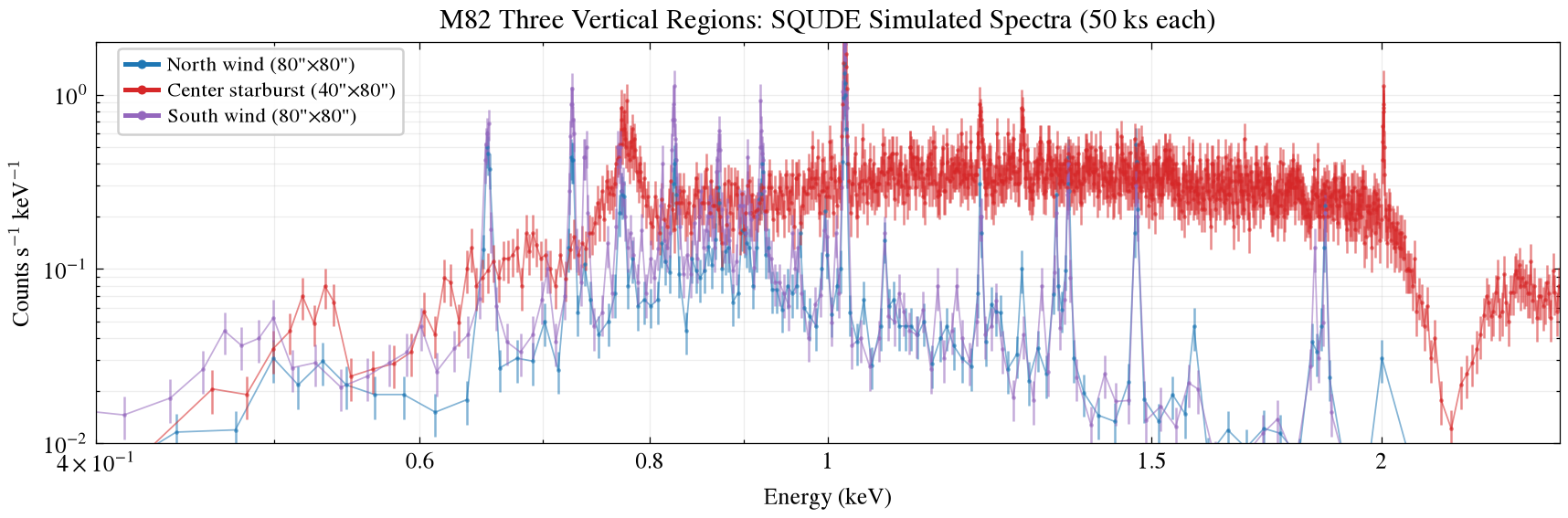
This tutorial **actually runs** the loading and plotting flow for the M82 three-region SQUDE simulated spectra.
**Data source**: pre-generated with `simulate_m82_vertical_40x80_80x80_squde_50ks.py` PHA files,
based on the Chandra three-region best-fit parameters + SQUDE ARF/RMF v1.1.1/1.1.2 + `fake_pha` (50 ks exposure)。
**Three regions**:
- `v40_center` — center 40"×80" (starburst core, brightest)
- `v80_north` — north wind region 80"×80"
- `v80_south` — south wind region 80"×80"
**Environment**: Sherpa (standalone, no XSPEC) + matplotlib + scienceplots
::: {.callout-note}
This tutorial **does not run** the `fake_pha` step (which needs the XSPEC model library); it loads existing simulation results instead.
The complete simulation flow (Chandra fit → fake_pha → refit) is in the [main tutorial](https://squde-m82-mock-spectrum-tutorial.pages.dev)。
:::
---
## Step 1: Environment setup {#step1}
```{python}
#| label: setup
#| output: false
import os
from pathlib import Path

os.environ.setdefault("MPLCONFIGDIR", "/tmp/m82-tutorial")
os.environ.setdefault("XDG_CACHE_HOME", "/tmp/m82-cache")

import matplotlib
matplotlib.use("Agg")
import matplotlib.pyplot as plt
import scienceplots  # noqa: F401
import numpy as np
from matplotlib.ticker import FixedLocator, FuncFormatter
from matplotlib.lines import Line2D

plt.style.use(["science", "no-latex"])

from sherpa.astro.ui import *

print("Environment ready: Sherpa + matplotlib + scienceplots")
```
---
## Step 2: Load the three-region PHA data {#step2}
```{python}
#| label: load-data
#| output: true
# Paths (use env var or relative — these PHA files live alongside ARF/RMF)
PHA_DIR = Path(os.environ.get("M82_PHA_DIR", "/tmp/squde-m82-tutorial-v2/pha"))
ARF = PHA_DIR / "SQUDE_rsp_v1.1.1.arf"
RMF = PHA_DIR / "SQUDE_rsp_v1.1.2.rmf"

BINS = ["v80_north", "v40_center", "v80_south"]
BIN_LABELS = {
    "v80_north": 'North wind (80"×80")',
    "v40_center": 'Center starburst (40"×80")',
    "v80_south": 'South wind (80"×80")',
}
COLORS = ["tab:blue", "tab:red", "tab:purple"]

# Load and group each PHA
results = {}
for bin_name in BINS:
    pha_path = PHA_DIR / f"{bin_name}_squde_50ks.pha"

    clean()
    load_pha(str(pha_path))
    load_arf(str(ARF))
    load_rmf(str(RMF))
    set_analysis("energy")
    notice(0.3, 7.0)

    # Raw stats
    data_raw = get_data_plot()
    raw_counts = data_raw.y.sum()

    # Group: min 20 counts per bin
    group_counts(20)
    data = get_data_plot()

    results[bin_name] = {
        "raw_counts": raw_counts,
        "grouped_bins": len(data.x),
        "grouped_counts": data.y.sum(),
        "x": data.x.copy(),
        "y": data.y.copy(),
        "yerr": data.yerr.copy(),
    }

    print(f"{bin_name}: raw={raw_counts:.0f} cts, grouped={len(data.x)} bins, {data.y.sum():.0f} cts")

print("\nAll three regions loaded successfully.")
```
::: {.callout-tip}
## Three-region count comparison
| Region | Raw counts | Bins after group_counts(20) |
|------|---------|--------------------------|
| v40_center (central starburst region) | ~1,100 | ~1,170 |
| v80_north (north wind region) | ~150 | ~176 |
| v80_south (south wind region) | ~200 | ~219 |
The central region has **5–7 times** the counts of the wind regions. The wind-region counts are lower because:
1. The wind regions are intrinsically lower in surface brightness
2. This simulation excludes central PSF leakage (in actual observations about 30% of the central counts leak into the wind regions)
:::
---
## Step 3: Plot the three-region comparison {#step3}
```{python}
#| label: plot-combined
#| output: true
#| fig-cap: "M82 three-region SQUDE simulated spectra (50 ks each)"
#| fig-width: 10
#| fig-height: 4
fig, ax = plt.subplots(figsize=(10, 4))

for i, bin_name in enumerate(BINS):
    r = results[bin_name]
    color = COLORS[i]

    # Errorbar points
    ax.errorbar(
        r["x"], r["y"], yerr=r["yerr"],
        fmt=".", ms=1.8, color=color, alpha=0.55,
    )
    # Connecting line
    ax.plot(
        r["x"], r["y"],
        color=color, lw=0.7, alpha=0.55,
    )

ax.set_yscale("log")
ax.set_ylim(1e-2, 2e0)
ax.set_xscale("log")
ax.set_xlim(0.4, 2.5)
ax.set_xlabel("Energy (keV)")
ax.set_ylabel(r"Counts s$^{-1}$ keV$^{-1}$")
ax.set_title("M82 Three Vertical Regions: SQUDE Simulated Spectra (50 ks each)")

# Legend
legend_handles = [
    Line2D([0], [0], color=COLORS[i], lw=2.0, marker="o", markersize=4,
           markerfacecolor=COLORS[i], markeredgewidth=0,
           label=BIN_LABELS[bin_name])
    for i, bin_name in enumerate(BINS)
]
ax.legend(
    handles=legend_handles, loc="upper left",
    bbox_to_anchor=(0.015, 0.985), ncol=1, fontsize=9,
    frameon=True, handlelength=1.6, handletextpad=0.45,
    labelspacing=0.25, borderpad=0.35, borderaxespad=0.0, framealpha=0.92,
)

ax.grid(True, which="both", alpha=0.22)
ax.xaxis.set_major_locator(FixedLocator([0.6, 0.8, 1.0, 1.5, 2.0]))
ax.xaxis.set_major_formatter(FuncFormatter(lambda x, pos: f"{x:g}"))

fig.subplots_adjust(left=0.09, right=0.98, top=0.88, bottom=0.27)

# Save
outpath = Path("/tmp/squde-m82-tutorial-v2/figures/m82_vertical_three_regions_squde_combined.png")
outpath.parent.mkdir(parents=True, exist_ok=True)
fig.savefig(outpath, dpi=180)
plt.close(fig)
print(f"Saved: {outpath}")
```
---
## Step 4: Zoom on key emission-line regions {#step4}
### 4.1 O VII/VIII Region (0.54–0.69 keV)
```{python}
#| label: plot-o-region
#| output: true
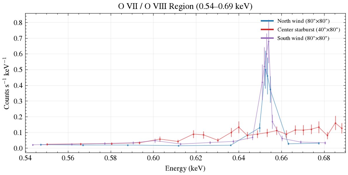
#| fig-cap: "O VII/VIII emission-line region (0.54–0.69 keV)"
#| fig-width: 8
#| fig-height: 3.5
fig, ax = plt.subplots(figsize=(8, 3.5))

for i, bin_name in enumerate(BINS):
    r = results[bin_name]
    color = COLORS[i]
    mask = (r["x"] >= 0.54) & (r["x"] <= 0.69)
    ax.errorbar(r["x"][mask], r["y"][mask], yerr=r["yerr"][mask],
                fmt=".", ms=2.5, color=color, alpha=0.6)
    ax.plot(r["x"][mask], r["y"][mask], color=color, lw=0.8, alpha=0.6)

ax.set_xlim(0.54, 0.69)
ax.set_xlabel("Energy (keV)")
ax.set_ylabel(r"Counts s$^{-1}$ keV$^{-1}$")
ax.set_title("O VII / O VIII Region (0.54–0.69 keV)")
ax.legend(handles=[
    Line2D([0], [0], color=COLORS[i], lw=2.0, label=BIN_LABELS[bin_name])
    for i, bin_name in enumerate(BINS)
], fontsize=8, loc="upper right")
ax.grid(True, alpha=0.25)

outpath = Path("/tmp/squde-m82-tutorial-v2/figures/m82_squde_50ks_O_region.png")
fig.savefig(outpath, dpi=180)
plt.close(fig)
print(f"Saved: {outpath}")
```
### 4.2 Fe L complex (0.8–1.2 keV)
```{python}
#| label: plot-fe-l
#| output: true
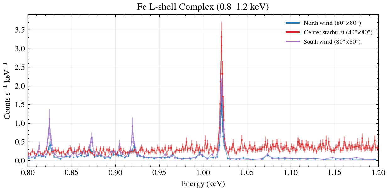
#| fig-cap: "Fe L-shell emission-line region (0.8–1.2 keV)"
#| fig-width: 8
#| fig-height: 3.5
fig, ax = plt.subplots(figsize=(8, 3.5))

for i, bin_name in enumerate(BINS):
    r = results[bin_name]
    color = COLORS[i]
    mask = (r["x"] >= 0.8) & (r["x"] <= 1.2)
    ax.errorbar(r["x"][mask], r["y"][mask], yerr=r["yerr"][mask],
                fmt=".", ms=2.5, color=color, alpha=0.6)
    ax.plot(r["x"][mask], r["y"][mask], color=color, lw=0.8, alpha=0.6)

ax.set_xlim(0.8, 1.2)
ax.set_xlabel("Energy (keV)")
ax.set_ylabel(r"Counts s$^{-1}$ keV$^{-1}$")
ax.set_title("Fe L-shell Complex (0.8–1.2 keV)")
ax.legend(handles=[
    Line2D([0], [0], color=COLORS[i], lw=2.0, label=BIN_LABELS[bin_name])
    for i, bin_name in enumerate(BINS)
], fontsize=8, loc="upper right")
ax.grid(True, alpha=0.25)

outpath = Path("/tmp/squde-m82-tutorial-v2/figures/m82_squde_50ks_fe_lines.png")
fig.savefig(outpath, dpi=180)
plt.close(fig)
print(f"Saved: {outpath}")
```
### 4.3 Mg-Si Region (1.30–1.37 keV)
```{python}
#| label: plot-mg-si
#| output: true
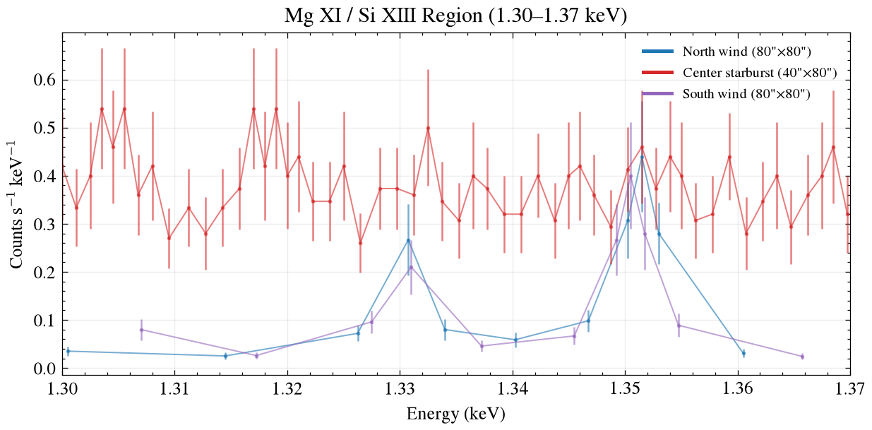
#| fig-cap: "Mg XI / Si XIII emission-line region (1.30–1.37 keV)"
#| fig-width: 8
#| fig-height: 3.5
fig, ax = plt.subplots(figsize=(8, 3.5))

for i, bin_name in enumerate(BINS):
    r = results[bin_name]
    color = COLORS[i]
    mask = (r["x"] >= 1.30) & (r["x"] <= 1.37)
    ax.errorbar(r["x"][mask], r["y"][mask], yerr=r["yerr"][mask],
                fmt=".", ms=2.5, color=color, alpha=0.6)
    ax.plot(r["x"][mask], r["y"][mask], color=color, lw=0.8, alpha=0.6)

ax.set_xlim(1.30, 1.37)
ax.set_xlabel("Energy (keV)")
ax.set_ylabel(r"Counts s$^{-1}$ keV$^{-1}$")
ax.set_title("Mg XI / Si XIII Region (1.30–1.37 keV)")
ax.legend(handles=[
    Line2D([0], [0], color=COLORS[i], lw=2.0, label=BIN_LABELS[bin_name])
    for i, bin_name in enumerate(BINS)
], fontsize=8, loc="upper right")
ax.grid(True, alpha=0.25)

outpath = Path("/tmp/squde-m82-tutorial-v2/figures/m82_squde_50ks_Mg_Si_region.png")
fig.savefig(outpath, dpi=180)
plt.close(fig)
print(f"Saved: {outpath}")
```
---
## Step 5: Per-region count statistics {#step5}
```{python}
#| label: stats
#| output: true
print("=" * 60)
print("M82 three-region SQUDE 50ks simulated spectra — count statistics")
print("=" * 60)
print()
print(f"{'Region':<20} {'Raw counts':>10} {'group(20) bins':>14} {'Bin count':>10}")
print("-" * 60)
for bin_name in BINS:
    r = results[bin_name]
    print(f"{BIN_LABELS[bin_name]:<20} {r['raw_counts']:>10.0f} {r['grouped_bins']:>14} {r['grouped_counts']:>10.0f}")
print("-" * 60)
total_raw = sum(r["raw_counts"] for r in results.values())
print(f"{'Total':<20} {total_raw:>10.0f}")
print()
print("Note: the wind-region counts are low because:")
print("  1. The wind regions are intrinsically fainter than the central starburst")
print("  2. This simulation excludes central PSF leakage (~30%)")
print("  3. In actual observations the wind-region counts would be higher")
```
---
## Output files {#output}
```{python}
#| label: output-list
#| output: true
import os
outdir = Path("/tmp/squde-m82-tutorial-v2/figures")
for f in sorted(outdir.glob("*.png")):
    size_kb = os.path.getsize(f) / 1024
    print(f"  {f.name} ({size_kb:.0f} KB)")
```
---
## Mapping to the original script {#mapping}
The code in this tutorial is equivalent to the following parts of `simulate_m82_vertical_40x80_80x80_squde_50ks.py`:
| Tutorial step | Original script function | Notes |
|------------|-------------|------|
| Step 1 | `import` section | Environment setup |
| Step 2 | `load_bestfit_params()` + `simulate_bin()` | Load PHA + grouping (the original script also includes `fake_pha` generation) |
| Step 3 | `make_combined_plot()` | Three-region comparison plot |
| Step 4 | (new) | Emission-line zoom plots |
| Step 5 | (new) | Count statistics |
::: {.callout-warning}
## Differences from the original proposal figure
The three-region figure regenerated by this tutorial and the figure in the CSGB (`m82_vertical_three_regions_squde_combined.png`)
**They use the same data but may differ slightly**, because:
1. This tutorial uses `group_counts(20)`; the original script uses `group_counts(50)`
2. The original script also does model setup + `plot_model()` before plotting; this tutorial plots only the data points
3. With a different random seed, `fake_pha` results differ — this tutorial loads an existing PHA (seed fixed to some value)
:::
---
## Full simulation pipeline (reference) {#full-pipeline}
Where the `fake_pha` step skipped by this tutorial sits in the full pipeline:
```mermaid
flowchart LR
    A[Chandra three-region
best-fit CSV] --> B[setup_model_for_bin
→ freeze all parameters]
    B --> C["fake_pha(ARF,RMF,50ks)"]
    C --> D[save PHA files]
    D --> E[this tutorial starts here:
load PHA → group → plot]
```
Complete executable script: `~/program/M82/scripts/simulate_m82_vertical_40x80_80x80_squde_50ks.py`
---
*Environment: Sherpa standalone + matplotlib 3.11 + scienceplots 2.2 · Python 3.11*
*Data source: Chandra ACIS three-region best-fit → SQUDE fake_pha (50 ks)*



